The case for high floor players: A thread.
When discussing team construction and the merits of a player there is always high variance production players and more consistent players. This thread is going to go in-depth into those players with some help from gambling and particles

NOTE: If you don't care about the simulation or models etc... I suggest reading part 7. The first 1-6 parts are pretty technical.

(1/18) First, we need to talk about quantum mechanics and probability distributions ( this will be light :). One of the earliest things you learn in quantum is probability distributions of the position of a particle. This qualifies as "the likelihood you'd find a particle there."

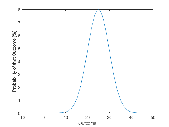
(2/18) Typically these distribtuions are "normal" or "Gaussian" if you're so inclined. These types of distributions exist everywhere: Heights, IQ, road kill, etc... Typically you'll see something like this (using arbitrary states to show curve trends):

(3/18) Now the trick with Quantum is we don't know the particles position. When we measure it, we "collapse" this curve to a very small point (though not exact but unimportant) and the result is a close approximation of that particles position.

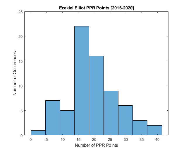
(4/18) This same concept can be directly applied to a player's fantasy points. Football player's fantasy production tends to result in a "gaussian" distribution of points. This can be broken by very low value players who produce rarely but an example is shown below for Zeke:

(5/18) The creation of a normal distribution relies on a player's average total scoring and the variance of said scoring (also known as mean and standard deviation). What this means is that a person with too much time on their hands could make a model of a fantasy season.

(6/18) While a fantasy season is long and it's hard to pull data from a single set, a modeled fantasy season could be run 1000 times over to test different data trends. If you DM me I can go into more on simulation methods but y'all just want to hear about FOOTBALL.

(7/18) Using what is known as a Monte Carlo Simulation, A 16 game season is simulated utilizing random number generation to account for variance in scoring. QB, RB, WR, TE, and FLX scoring are all approximated using the lower Tier 1 players at each position. Results are shown

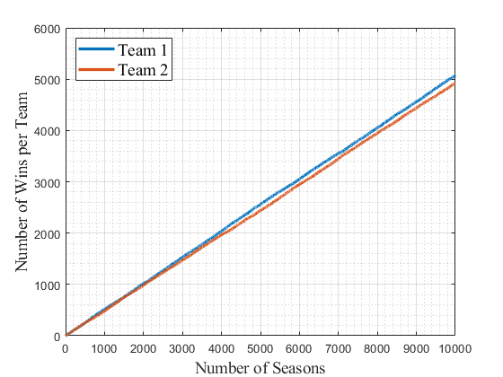
(8/18) Using a 16 week season, 2 teams are constructed using a typical format 1QB, 2RB, 2WR, 1TE, 2FLX, 1SF (Assumed QB). Each team is also fed the same results for mean and std. deviation. At the end of a season, the team with the most wins gets 1 point. A tie is half for both.

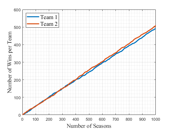
(9/18) As is shown, with everything kept the same, the results as expected are pretty equal. Both teams winning ~500 games. Any deviation is due to randomness which is inherent to the sim. Now is where the fun begins.

(10/18) The difference between a "High Variance" and "High Floor" player depends on what is changed, their std. deviation or their average. So a "high variance" player has a higher std. deviation. A "high floor player" has a higher average. So let's see how that affects the sim.

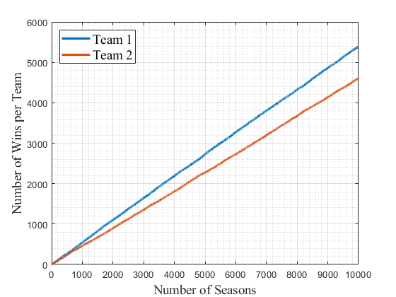
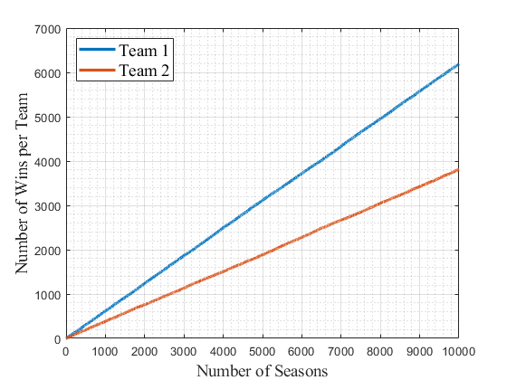
(11/18) If one were to increase the average production of an RB by just 1 point on team 1, we can quantify that effect. The result is a HUGE advantage for Team 1. With a nearly 7% advantage to win a season. And 775 extra wins over 10k seasons. This is 1 ppg on 1 RB.

(12/18) Now let's do the same for the std. Deviation: adding 3 points of std. deviation onto that same player. but put the averages back to normal (This will be a HIGHLY volatile RB with high upside but a lower floor.) The result is only a 1.5% advantage for Team 1.

(13/18) The reason for this is the shape of the distribution of a Normal Curve. Because it is symmetric, increasing std. Dev will increase the likelihood of high scoring games but increase the likelihood of low scoring as well. Averaging each other out.

(14/18) However, increasing the average will shift that whole distribution. Giving an advantage for the high floor player over the high variance. It takes a while to increase the variance before a player truly starts showing the effects.

(15/18) If we increase the difference to say an increase in the average by 3 points (the difference between drafting Nick Chubb and Josh Jacobs last year) the result is even more baffling. Nick Chubb winning nearly 2500 more seasons to a nearly 25% advantage ALL ELSE EQUAL.

(16/18) So why do high variance players still get picked? Kamara, CMC, etc... are fantasy winners year after year. This is because of the RB position's reliance on the opportunity. These players have a floor that bolsters that high variance, (thus making that curve asymmetric).

(17/18) This thread is certainly not complete as it still needs to take into account injuries/opportunity share but it steps one of a simulator I'm working on. The point is to show that all things else considered, high variance wins games, high floor wins seasons.

(18/18) Thank you so much for reading. This took a lot of time and editing. I appreciate you making it this far. Feel free to DM me if you have questions about the model or suggestions for additions. Thank y'all as always!