Thanks so much, Jen, for tweeting about our paper!

A brief thread diving into the econometrics black box: 1/N https://twitter.com/jenniferdoleac/status/1357317831084367874

Social scientists are often interested in policies that are adopted by different units at different times.

States pass laws at different times; employees get trainings at different times; etc. 2/N

There’s been a lot of great work recently on how to estimate treatment effects under a parallel trends assumption btwn cohorts treated at diff times. Two-way FE models give you a weird weighted average, but there are really good alternatives! CC @pedrohcgs @CdeChaisemartin 3/N

However, in many cases, we either explicitly can randomize the rollout of treatment *or* we justify parallel trends by arguing that treatment timing is quasi-randomly assigned. 4/N

In this paper we think about how we can more efficiently estimate treatment effects if we’re willing to make the assumption of random treatment timing (which is stronger than parallel trends). 5/N

How does it work? To gain intuition, let’s take a brief detour from the staggered set-up. Suppose I have an experiment where I randomly give some people a job training program. 6/N

Let:

Y = earnings after experiment

D= treatment status

X = individual covariates 7/N

You might want to use the individual covariates to try to gain more precision in your treatment effects estimates. You’d probably run a regression like:

Y = D tau + X beta + e

8/N

You’d also probably think it’s pretty weird if I told you that instead of doing this, without looking at the data, I was going to impose that the coefficient on X was equal to 1.

But if X is pre-treatment earnings, that’s exactly what the DID estimator is doing!! 9/N

Check it out:

If

Y = Y_t
X = Y_{t-1}

Then

Y = D tau + X * 1 + e

If and only if

Y_t - Y_{t-1} = D tau + e

10/N

So the simple DiD estimator in this case is like a regression adjustment estimator that assumes that we knew that the coefficient was exactly 1. Weird, right?

You’d think that you could do better by estimating that coeff from the data. And you would be right…almost! 11/N

Actually, if you want to guarantee we get a more precise estimate we need to run a separate regression of Y on X for the treated and control group, and then combine those coefficients in the end.

This is for technical reasons discussed in the papers referenced here: 12/N

https://twitter.com/jondr44/status/1357766518021345282?s=20

Don’t worry about that too much. Under homogeneous effects, the usual OLS regression would be just fine, and this is a tweak to allow for a heterogeneity so that cov(Y(1),X) and cov(Y(0),X) may not be the same 13/N

Okay, now back to staggered timing!

Suppose that we have 3 periods, t=1,2,3.

Some units are randomly treated at t=2, and some at t=3.

14/N

If we look at the outcome in period 2, we have something very similar to the cross-sectional experiment we just thought about. Some units are randomly treated, some aren’t yet treated, and we have pre-treatment outcomes for both groups. 15/N

If we just cared about the avg effect in period 2, by the same logic as above, we could get a more efficient estimate by allowing the data to tell us what coefficient to put on lagged outcomes instead of imposing beta =1. 16/N

As it turns out, all of the modern staggered DiD tools to deal with weird weighting basically aggregate a bunch of simple DiDs of this type. In fact, the usual TWFE estimator can be thought of as aggregating simple DiDs too, although in a weird, non-convex way! 17/N

So the basic idea of our paper is, instead of running these DiDs and aggregating them, we do a more efficient estimation that chooses the weight on lagged outcomes from the data. Intuitively, we put more weight on lagged outcomes if they better predict current outcomes 18/N

It’s actually a bit more complicated than that, since we have to account for the covariance between the simple 2-period estimates in choosing the optimal weights, but we take care of those details in the paper 19/N

We find that efficiently controlling for lagged outcomes, instead of imposing a coef of 1, can yield substantial reductions in SEs. 20/N

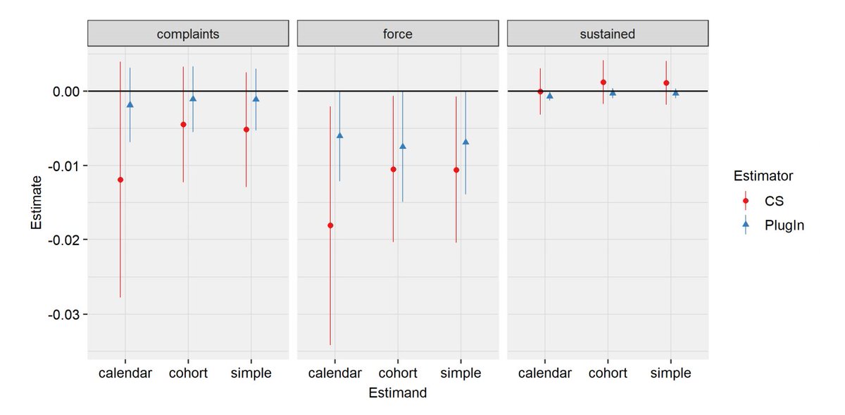
Here’s a comparison of CIs between our procedure and the state-of-the-art in Callaway and Sant’Anna when applied to our criminal justice application.

Our CIs are between 30% and 500% (no typo!) times as small! 21/N

We can’t guarantee such gains in all cases, but we find in simulations they tend to be larger i) with many periods, and ii) when serial correlation of the outcome is far from 1. 22/N

We might do another thread on the application, since it’s potentially of interest to criminal justice folks on its own, but that’s all for now!

Paper: https://arxiv.org/pdf/2102.01291.pdf
R package: https://github.com/jonathandroth/staggered

N/N