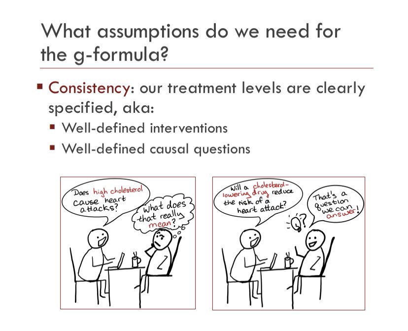
Turns out I’ve never actually explained the g-formula #onhere, even though I tweet about quite a bit, and it’s a vital part of my #causalinference toolkit & helps shape my whole approach doing science.
So, b/c it’s Sunday & I’m bored, let’s nerd out a bit. Ready? https://twitter.com/epiellie/status/1355957990176784384
So, b/c it’s Sunday & I’m bored, let’s nerd out a bit. Ready? https://twitter.com/epiellie/status/1355957990176784384
Before we get into the details of the g-formula, we need to step back & talk about what #causalinference is.
Simply put, causal inference is the science of getting a reliable & believable answer to the question “what will happen in the world if I do A instead of B?”
Simply put, causal inference is the science of getting a reliable & believable answer to the question “what will happen in the world if I do A instead of B?”
Say we wanted to know how many fewer people would have heart attacks if everyone was vegetarian compared to if everyone ate meat.
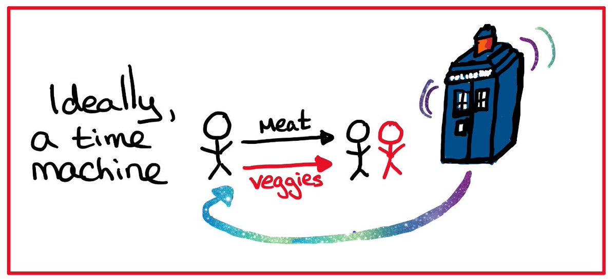
If we had a time machine, we could feed people one diet, see what happens, and then go back & do it over with the other diet.
If we had a time machine, we could feed people one diet, see what happens, and then go back & do it over with the other diet.
Now, IDK about you, but I don’t have a time machine and neither do any scientists I know.
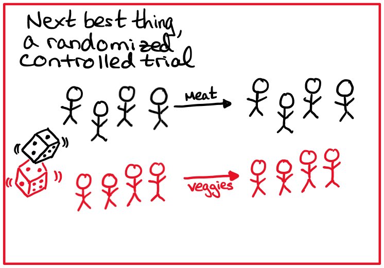
Another option, and what many consider the next best thing, is to do a controlled experiment or randomized controlled trial.
To do this, you create 2 groups of people with the same heart attack risk, feed some veggies & others meat, and see what happens.
To do this, you create 2 groups of people with the same heart attack risk, feed some veggies & others meat, and see what happens.
Assuming you were right the groups had the same risk to start with, & assuming they all eat what you tell them to, & assuming they all tell you let if they have a heart attack, then this is pretty much as good as a time machine.
Now that might seem simple, but it’s actually a pretty hard set of requirements to meet.
Often people wont do what you ask them to, or they decide not to stay in your study so you don’t know what happens to them, or the thing you want to know about is dangerous.
Often people wont do what you ask them to, or they decide not to stay in your study so you don’t know what happens to them, or the thing you want to know about is dangerous.
This might seem like a problem but for nerds like me this is where things start to get exciting!
The big question is: why is it that an experiment mimics a time machine & how can we make non-experimental data mimic a time machine too?
The big question is: why is it that an experiment mimics a time machine & how can we make non-experimental data mimic a time machine too?
Okay, don’t freak out but I’m gonna use some algebra notation now.
Let’s start with some definitions.
Let’s start with some definitions.
A is going to mean the thing I want to change (variously called the cause, exposure, treatment, independent variable). It will have two values: a and a’
Y is going to be the thing I think might change BECAUSE I changed A (variously called the outcome, effect, dependent variable)
Y is going to be the thing I think might change BECAUSE I changed A (variously called the outcome, effect, dependent variable)
We can draw a picture of this
(the technical name for this picture is a “directed acyclic graph” or “DAG” but thats a whole other #tweetorial)
(the technical name for this picture is a “directed acyclic graph” or “DAG” but thats a whole other #tweetorial)
In an experiment, we get to change A directly and see what happens to Y. This is the same thing we get to do if we have a time machine with ONE key difference!
The time machine lets us change A more than once for each person but the experiment only lets us vary A between groups.
The time machine lets us change A more than once for each person but the experiment only lets us vary A between groups.
So, with a time machine, we could talk about what anyones Y is (or will be) when they are given A,
but with an experiment we can only talk about what the *expected* Y is (or will be) for *some group* when *some group* is given A.
but with an experiment we can only talk about what the *expected* Y is (or will be) for *some group* when *some group* is given A.
We can write what we learn from the experiment in two ways:
The expected Y when YOUR group *does* get a is: E[Y|a]
•this is math for “expected Y when A is a”
The expected Y when ANY group *will be* given a is: E[Y^a]
•this is math for “expected Y if A is a”
The expected Y when YOUR group *does* get a is: E[Y|a]
•this is math for “expected Y when A is a”
The expected Y when ANY group *will be* given a is: E[Y^a]
•this is math for “expected Y if A is a”
The difference between E[Y|a] and E[Y^a] is the heart of almost all weird, confusing, or down right laughable science you’ve ever read.
You might have heard “correlation is not causation”? It’s a simple way of saying that E[Y|a] is not (always) equal to E[Y^a]
You might have heard “correlation is not causation”? It’s a simple way of saying that E[Y|a] is not (always) equal to E[Y^a]
But “correlation is not causation” is only half the story, because whenever A causes Y, A will also be correlated with Y.
That is, _causation_ *is* correlation!
What this means is that *sometimes* correlation must be causation too.

That is, _causation_ *is* correlation!
What this means is that *sometimes* correlation must be causation too.


Okay, some of you are probably starting to wondering when the heck I’m going to get to the point of all this, which I said was the g-formula.
Well my friends, I’m already there!
The g-formula tells us how to get causation from correlation, i.e. how to learn E[Y^a] from E[Y|a]
Well my friends, I’m already there!
The g-formula tells us how to get causation from correlation, i.e. how to learn E[Y^a] from E[Y|a]
But I kinda lied. I need to talk about one more problem before we get to the g-formula.
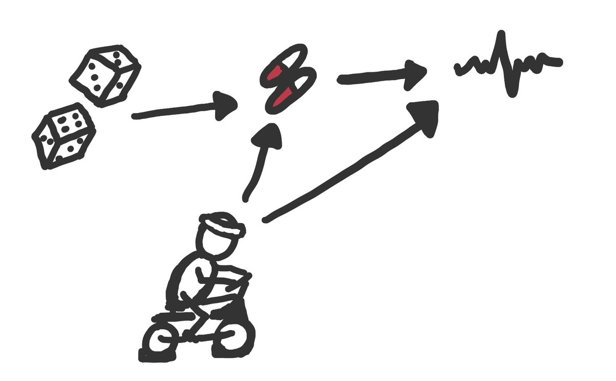
In our experiment, let’s say we tell people to take some medicine or placebo and want to know how this changes their heart function. The picture below shows how these things might be related
In our experiment, let’s say we tell people to take some medicine or placebo and want to know how this changes their heart function. The picture below shows how these things might be related
The dice are randomization (let’s call this Z), the pills are the medicine (our A), and the heart rate is heart function (our Y).
Now, we can look at our data and easily calculate E[Y|Z=z] by getting the average heart rate in people randomized to group Z=z
Now, we can look at our data and easily calculate E[Y|Z=z] by getting the average heart rate in people randomized to group Z=z
The magic of randomization is that it makes the two groups of people asked to take A (a & a’) equal at the start of our study.
This means, if we hadnt given anyone any pills then the average heart rate in the Z=z group would be the same as what the average in the Z=z’ group.
This means, if we hadnt given anyone any pills then the average heart rate in the Z=z group would be the same as what the average in the Z=z’ group.
Even better, it *also* means that if everyone does what we ask, then the average heart rate in the Z=z group after they get A=a, is the same as what the average heart rate *would have been* for the Z=z’ group if we had given them A=a instead of A=a’!
Going back to our algebra, randomization means E[Y|z]=E[Y^z]
Correlation *is* causation, for a randomized controlled trial!
What we learn by randomizing some to a & others to a’ *is what we would have learned if we used a time machine to randomize EVERYONE to a & then to a’
Correlation *is* causation, for a randomized controlled trial!
What we learn by randomizing some to a & others to a’ *is what we would have learned if we used a time machine to randomize EVERYONE to a & then to a’
In a randomized trial, E[Y|z]=E[Y^z] is the general formula for how to convert the data you have (E[Y|z]) into the data you would like to know about (E[Y^z])
That is, for this special case, E[Y|z]= E[Y^z] is the g-formula!
That is, for this special case, E[Y|z]= E[Y^z] is the g-formula!
Okay, I know what you’re thinking.
You’re thinking, hey @epiellie, this seems dumb. Why do we need a special name for E[Y|z] = E[Y^z] and why did you write a whole tweet thread about it???
Don’t worry, we’re just getting started! But I’m outta space, so stay tuned for part 2!
You’re thinking, hey @epiellie, this seems dumb. Why do we need a special name for E[Y|z] = E[Y^z] and why did you write a whole tweet thread about it???
Don’t worry, we’re just getting started! But I’m outta space, so stay tuned for part 2!
So, okay, in a perfect experiment
E[Y|z]=E[Y^z] is the only equation we need to know.
But, when we’re working with humans no experiment is perfect and as we said before, lots of times we can’t experiment anyway.
The next step is to figure out how experiments can go wrong.
E[Y|z]=E[Y^z] is the only equation we need to know.
But, when we’re working with humans no experiment is perfect and as we said before, lots of times we can’t experiment anyway.
The next step is to figure out how experiments can go wrong.
The most likely thing to go wrong in your randomized trial is that not everyone actually does what you ask them to
(scientists call this “non-adherence” or “non-compliance” and I know those words suck but there aren’t really any alternatives )
)
Consider this picture
(scientists call this “non-adherence” or “non-compliance” and I know those words suck but there aren’t really any alternatives
 )
) Consider this picture

In this picture, there are two reasons a person might take the medication:
They were randomized to the medication group & asked to take it by the trial team.
Or, they are super healthy fitness buffs and asked for these meds from their regular doctor b/c they wanna try them
They were randomized to the medication group & asked to take it by the trial team.
Or, they are super healthy fitness buffs and asked for these meds from their regular doctor b/c they wanna try them
Is that a problem? As with everything in epidemiology the only correct answer is: it depends!
(That’s why it’s our official #epitwitter slogan!)
(That’s why it’s our official #epitwitter slogan!)
So, what does it depend on?
In this case, the key question is whether exercise (the other cause of getting the meds) is also good for your heart function.
If it is, then we have a problem.
In this case, the key question is whether exercise (the other cause of getting the meds) is also good for your heart function.
If it is, then we have a problem.

It’s *still* true that by randomizing, we can learn what the expected heart function for the whole group from looking at the heart function of the Z=z group.
But in our perfect trial, we could conclude that a difference between the expected heart function if everyone was randomized to Z=z versus if everyone had been randomized to Z=z’ was *actually* because of the difference in A between groups.
That is E[Y^z]-E[Y^z’]=E[Y^a]-E[Y^a’]
That is E[Y^z]-E[Y^z’]=E[Y^a]-E[Y^a’]
This quantity, E[Y^z]-E[Y^z’]=E[Y^a]-E[Y^a’], is the “causal effect”.
That is, it is the answer to our original question “how does Y change when I do a compared to a’”
That is, it is the answer to our original question “how does Y change when I do a compared to a’”
But in this new trial, where some people make their own choices, we can no longer attribute any differences between what happens to the Z=z group and what happens to the Z=z’ group to their different medication use.
That is, E[Y^z]-E[Y^z’] is NOT equal to E[Y^a]-E[Y^a’] anymore
That is, E[Y^z]-E[Y^z’] is NOT equal to E[Y^a]-E[Y^a’] anymore
Let’s introduce another letter to our algebra: L
L is going to mean any and everything else in the world that we know makes A change and has an impact on Y.
Just like exercise in this example
L is going to mean any and everything else in the world that we know makes A change and has an impact on Y.
Just like exercise in this example

So, we have a problem. Does that mean all is lost?
No! This is where the real beauty of the g-formula starts to show.
No! This is where the real beauty of the g-formula starts to show.
If we want to know how we should expect Y to change when we change A, but Y and A are both also changed by that pesky other thing L, then the solution is conceptually simple:
We can use math make our data mimic what would have happened if L didn’t also cause A!
We can use math make our data mimic what would have happened if L didn’t also cause A!
We want to find out what to expect Y to be, if everyone got medicine a. So our goal is to learn E[Y^a].
In our data, there are some different numbers we could calculate: E[Y|z], E[Y|z,a], E[Y|z,a,l], and E[Y|a]
In our data, there are some different numbers we could calculate: E[Y|z], E[Y|z,a], E[Y|z,a,l], and E[Y|a]
Before, E[Y|z] was all we needed. But now, it’s not good enough, because we want to know about *taking* the medicine, not about being *asked* to take the medicine.
What about E[Y|A]? Why don’t we just calculate this?
This is where our old friend, correlation is not causation, comes in.
This is where our old friend, correlation is not causation, comes in.
Because exercise affects taking the medicine AND heart rate, if we just compare people who do & dont take the medicine, we would see a difference in heart rate between these groups EVEN IF the medicine does nothing!
E[Y|a] is NOT equal to E[Y^a] because L is a “confounder”.
E[Y|a] is NOT equal to E[Y^a] because L is a “confounder”.
That leaves us with two options: E[Y|z,a] and E[Y|z,a,l]. Can we learn anything from these? Yes!
E[Y|z,a] has the problems of both E[Y|a] and E[Y|z] but also the benefits of both, and we could use it to answer our question. But, this only works sometimes! So, lets skip it.
E[Y|z,a] has the problems of both E[Y|a] and E[Y|z] but also the benefits of both, and we could use it to answer our question. But, this only works sometimes! So, lets skip it.
We’re looking for a General formula that works all the time, after all!
And this last option, E[Y|z,a,l], is going to help us!
To understand how, a quick ice cream break
And this last option, E[Y|z,a,l], is going to help us!
To understand how, a quick ice cream break
Here’s a random fact for you: if you track them over time, the way amount of ice cream being eaten in a city changes is very similar to the way that the amount of petty crime changes.
Does eating ice cream make people commit crimes?!
Does eating ice cream make people commit crimes?!
No! What’s really going on is that both ice cream eating & petty crime arrests are higher in the summer!
If we don’t account for season, we think ice cream & crime are related. But if we account for season, then we see they are completely independent!
If we don’t account for season, we think ice cream & crime are related. But if we account for season, then we see they are completely independent!
We can do the same thing when we want to understand our trial! We need to account for exercise when we compare medication use and heart rate.
An easy way to account for something is what’s called “stratification”.
In the ice cream example, this would mean comparing ice cream & crime in summer separately from winter. If we want, we can then average those answers together to get one answer for the whole year.
In the ice cream example, this would mean comparing ice cream & crime in summer separately from winter. If we want, we can then average those answers together to get one answer for the whole year.
In the trial, we can do the same thing.
We calculate the expected Y for people who take the medication separately based on whether they exercise or not, and then average the answer!
We calculate the expected Y for people who take the medication separately based on whether they exercise or not, and then average the answer!
Now, because exercising isnt 50/50 we dont just want to do a simple average. Instead we use a weighted average, based on what percent of people assigned to medicine a also exercise.
We can write that percentage using math as: P(L=1|Z=z)
We can write that percentage using math as: P(L=1|Z=z)
So, we now have our g(eneral)-formula!
E[Y^a] = E[Y|a,z,L=l]*P(L=l|Z=z)
It’s just a weighted average of what happened in our trial, but because L is the only other variable that causes A and Y, accounting for it lets us know what would have happened if it hadnt been a problem!
E[Y^a] = E[Y|a,z,L=l]*P(L=l|Z=z)
It’s just a weighted average of what happened in our trial, but because L is the only other variable that causes A and Y, accounting for it lets us know what would have happened if it hadnt been a problem!
Part 3! (I warned you I had a lot to say about the g-formula!)
We know how to do two really basic versions of the g-formula now.
E[Y^z]=E[Y|z] when there are no other joint causes of Z & Y, and
E[Y^a]=E[Y|a,z,l]*P(l|z) when we have a less than perfect trial.
We know how to do two really basic versions of the g-formula now.
E[Y^z]=E[Y|z] when there are no other joint causes of Z & Y, and
E[Y^a]=E[Y|a,z,l]*P(l|z) when we have a less than perfect trial.
One step further is that we don’t randomize at all. We simply let people decide on their own to do a or a’ and then ask why.
That might look like this
Now, our g-formula is:
E[Y^a]=E[Y|a,l]*P(l)
All the same reasoning applies, but Z isn’t relevant so we don’t need it!
That might look like this

Now, our g-formula is:
E[Y^a]=E[Y|a,l]*P(l)
All the same reasoning applies, but Z isn’t relevant so we don’t need it!
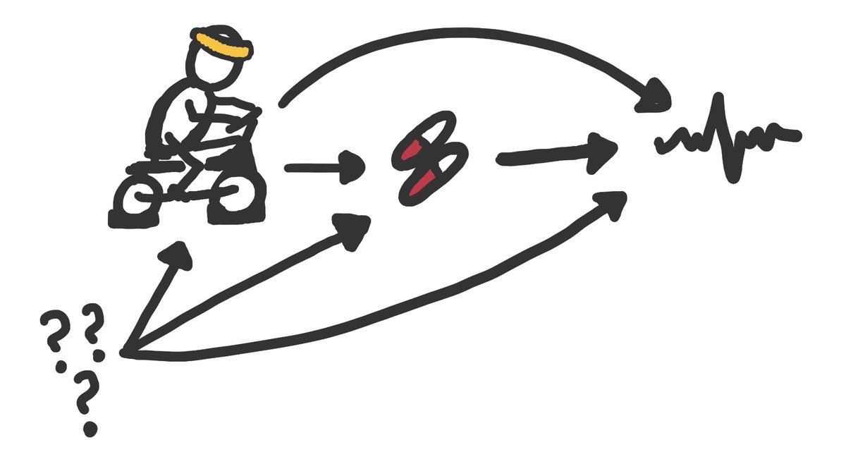
What about there were 2 reasons people might take meds & they both affect heart function?
If we don’t know what they all are, we’re in trouble! But we can still write out a g-formula.
If we don’t know what they all are, we’re in trouble! But we can still write out a g-formula.
We can use the picture to help figure out what our g-formula should look like.
Because there are arrows from L and ??? to A and Y, we need to know: E[Y|a,L,???]
Because there are arrows from L and ??? to A and Y, we need to know: E[Y|a,L,???]
Then, because there is an arrow from ??? to L we need to know P(L|???)
Because ??? is in E[Y|a,L,???] we also need to know about the percentage of people with ???, but there are no arrows into it. So we only need P(???).
Because ??? is in E[Y|a,L,???] we also need to know about the percentage of people with ???, but there are no arrows into it. So we only need P(???).
As your data get more complicated, so does your g-formula.
But this basic process works no matter how many L-type variables you have and no matter how complicated the changes you want to compare are!
But this basic process works no matter how many L-type variables you have and no matter how complicated the changes you want to compare are!
Things get complicated to calculate pretty quickly though, but there are many ways to handle that.
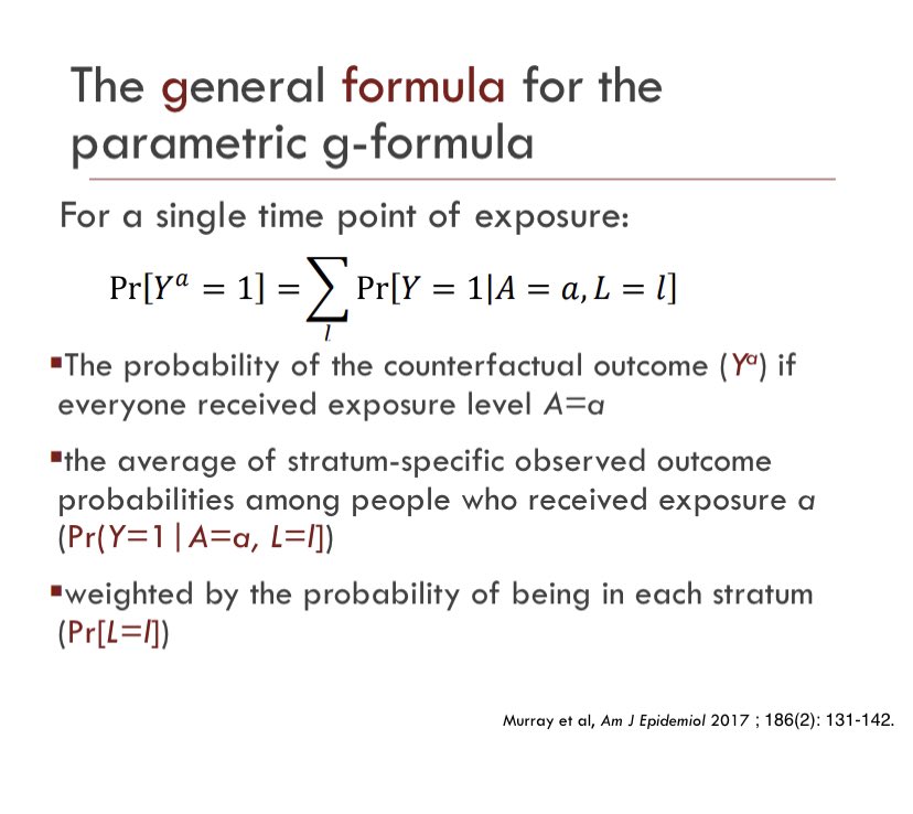
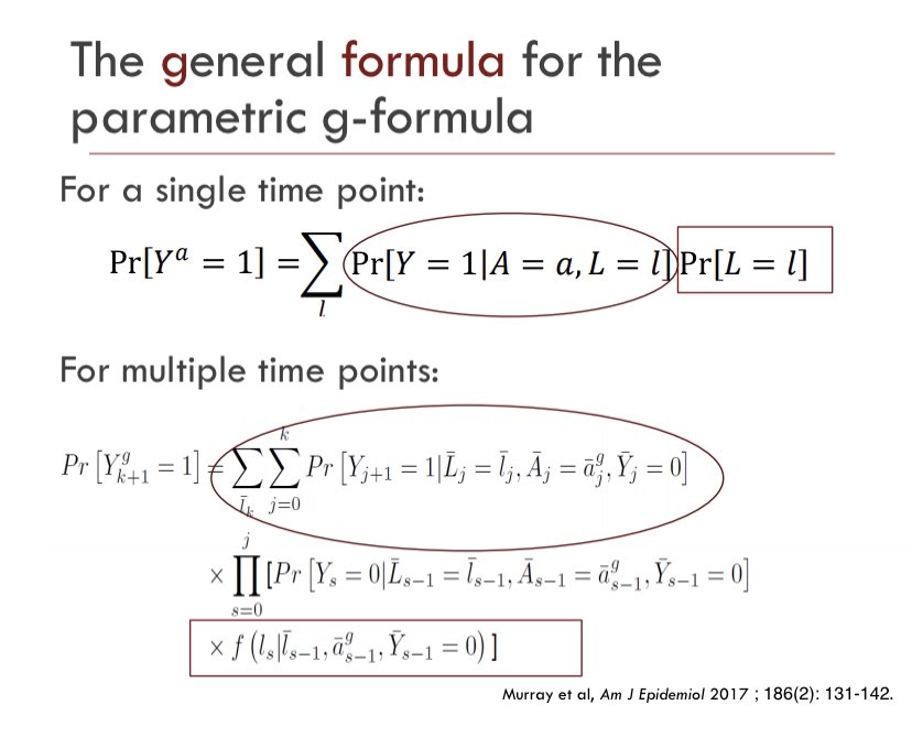
One way is to incorporate regression modeling. Instead of calculating each bit by hand, we can make some (parametric) modeling assumptions. We call that the parametric g-formula.
One way is to incorporate regression modeling. Instead of calculating each bit by hand, we can make some (parametric) modeling assumptions. We call that the parametric g-formula.
The technical details of this are less important than understanding the WHY of it all though.
Because you can spend your time calculating E[Y^a]=E[Y|a,l]*P(l) but if that ??? exists, then it wont actually equal E[Y^a]!
You would need E[Y|a,L,???]*P(L|???)*P(???) instead.
Because you can spend your time calculating E[Y^a]=E[Y|a,l]*P(l) but if that ??? exists, then it wont actually equal E[Y^a]!
You would need E[Y|a,L,???]*P(L|???)*P(???) instead.
So, what needs to be true for your g-formula to be the right one?
At minimum, the following 3 things

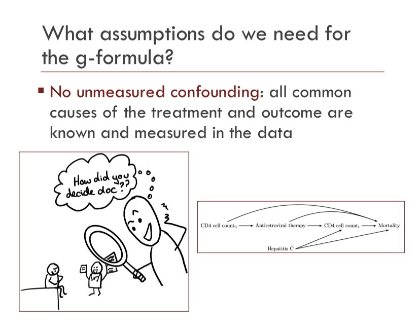
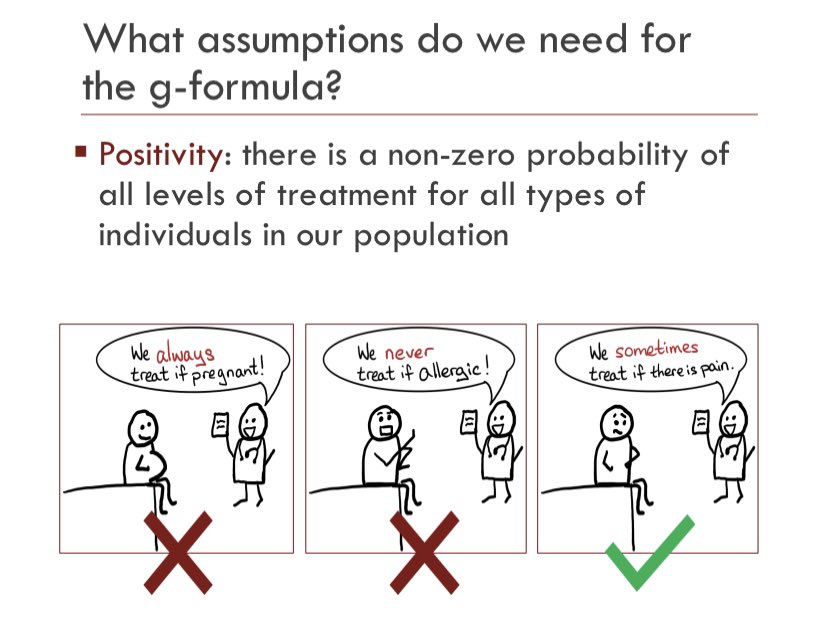
(1) You know all the shared causes, (2) everyone is eligible to get a & a’, and (3) you’ve asked a good causal question!
At minimum, the following 3 things


(1) You know all the shared causes, (2) everyone is eligible to get a & a’, and (3) you’ve asked a good causal question!
And that’s it. The basics of the g-formula.
Hope you enjoyed it

Hope you enjoyed it


 Read on Twitter




![The dice are randomization (let’s call this Z), the pills are the medicine (our A), and the heart rate is heart function (our Y).Now, we can look at our data and easily calculate E[Y|Z=z] by getting the average heart rate in people randomized to group Z=z The dice are randomization (let’s call this Z), the pills are the medicine (our A), and the heart rate is heart function (our Y).Now, we can look at our data and easily calculate E[Y|Z=z] by getting the average heart rate in people randomized to group Z=z](https://pbs.twimg.com/media/EtFs88jWMAIlTj1.jpg)
![Going back to our algebra, randomization means E[Y|z]=E[Y^z]Correlation *is* causation, for a randomized controlled trial! What we learn by randomizing some to a & others to a’ *is what we would have learned if we used a time machine to randomize EVERYONE to a & then to a’ Going back to our algebra, randomization means E[Y|z]=E[Y^z]Correlation *is* causation, for a randomized controlled trial! What we learn by randomizing some to a & others to a’ *is what we would have learned if we used a time machine to randomize EVERYONE to a & then to a’](https://pbs.twimg.com/media/EtFs-dVXUAM8t8k.jpg)
![Going back to our algebra, randomization means E[Y|z]=E[Y^z]Correlation *is* causation, for a randomized controlled trial! What we learn by randomizing some to a & others to a’ *is what we would have learned if we used a time machine to randomize EVERYONE to a & then to a’ Going back to our algebra, randomization means E[Y|z]=E[Y^z]Correlation *is* causation, for a randomized controlled trial! What we learn by randomizing some to a & others to a’ *is what we would have learned if we used a time machine to randomize EVERYONE to a & then to a’](https://pbs.twimg.com/media/EtFs-dlXIAAZVNA.jpg)
![So, okay, in a perfect experiment E[Y|z]=E[Y^z] is the only equation we need to know. But, when we’re working with humans no experiment is perfect and as we said before, lots of times we can’t experiment anyway. The next step is to figure out how experiments can go wrong. So, okay, in a perfect experiment E[Y|z]=E[Y^z] is the only equation we need to know. But, when we’re working with humans no experiment is perfect and as we said before, lots of times we can’t experiment anyway. The next step is to figure out how experiments can go wrong.](https://pbs.twimg.com/media/EtF4m_KXcAAGnfM.jpg)



![We want to find out what to expect Y to be, if everyone got medicine a. So our goal is to learn E[Y^a].In our data, there are some different numbers we could calculate: E[Y|z], E[Y|z,a], E[Y|z,a,l], and E[Y|a] We want to find out what to expect Y to be, if everyone got medicine a. So our goal is to learn E[Y^a].In our data, there are some different numbers we could calculate: E[Y|z], E[Y|z,a], E[Y|z,a,l], and E[Y|a]](https://pbs.twimg.com/media/EtF4qfPXYAEG_Ot.jpg)
![Before, E[Y|z] was all we needed. But now, it’s not good enough, because we want to know about *taking* the medicine, not about being *asked* to take the medicine. Before, E[Y|z] was all we needed. But now, it’s not good enough, because we want to know about *taking* the medicine, not about being *asked* to take the medicine.](https://pbs.twimg.com/media/EtF4qwoW8AYRBxe.jpg)
![Before, E[Y|z] was all we needed. But now, it’s not good enough, because we want to know about *taking* the medicine, not about being *asked* to take the medicine. Before, E[Y|z] was all we needed. But now, it’s not good enough, because we want to know about *taking* the medicine, not about being *asked* to take the medicine.](https://pbs.twimg.com/media/EtF4qxBW4AAvjqH.jpg)

![One step further is that we don’t randomize at all. We simply let people decide on their own to do a or a’ and then ask why.That might look like this Now, our g-formula is:E[Y^a]=E[Y|a,l]*P(l)All the same reasoning applies, but Z isn’t relevant so we don’t need it! One step further is that we don’t randomize at all. We simply let people decide on their own to do a or a’ and then ask why.That might look like this Now, our g-formula is:E[Y^a]=E[Y|a,l]*P(l)All the same reasoning applies, but Z isn’t relevant so we don’t need it!](https://pbs.twimg.com/media/EtF-wp0XcAAku0a.jpg)
![We can use the picture to help figure out what our g-formula should look like.Because there are arrows from L and ??? to A and Y, we need to know: E[Y|a,L,???] We can use the picture to help figure out what our g-formula should look like.Because there are arrows from L and ??? to A and Y, we need to know: E[Y|a,L,???]](https://pbs.twimg.com/media/EtF-xRrXUAMaGO3.jpg)
![Putting it all together, our new g-formula is:E[Y^a]=E[Y|a,L,???]*P(L|???)*P(???)Kinda cool, huh? Putting it all together, our new g-formula is:E[Y^a]=E[Y|a,L,???]*P(L|???)*P(???)Kinda cool, huh?](https://pbs.twimg.com/media/EtF-xpOXAAYw7-u.jpg)
