This came to my att'n a few hrs ago and it had an odd air of familiarity to it...until I realized here is a very good example of the Frechet-Hoeffding bounds in real life These bounds (which I'm kinda obsessed with) state that the marginal distributions of two variables place 1/6 https://twitter.com/jean_twenge/status/1333809422947155968
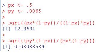
bounds on how large the correlation between them can be. For the case of binary data (treated/non-treated VS sick/not-sick) these bounds have been known since the 60s (we show the more general version in https://doi.org/10.1177/0013164420903770) and the upper bound looks like this: 2/6
With the data provided to build the 2x2 contingency table, the proportion of 'treated', px , is 0.5 and the proportion of 'got sick', py, is .0065 so if one checks the potential upper bound one can see that the maximum possible theoretical correlation for this data is.08 3/6
Although it is (correctly) pointed out in the thread that psych relies a bit too much on the correlation coefficient r, this problem has an old history in psychometrics. I'd say that a psychometrically-inclined psychologist would probably go for the 'quick-and-dirty' fix of 4/6
using 'max phi'. Which is really just finding the maximum possible phi coefficient (Pearson's r for binary data) and dividing one's estimated phi by max phi. So, in this case, .07/.08 = .875 and that's what one interprets. Max phi has been faced out by other coeffs these days 5/6
but I really liked this real-life scenario to sort of put it out there that without knowing the distributions of the variables we are correlating, we are missing out on a lot of potentially good information 6/6

 Read on Twitter


